The following is a quotation from a previous article in this series: “Science is almost always able to provide answers to questions about observed phenomena. Consider as examples: “Why are honeycombs made up of regular hexagons?”, “Why are snowflakes sometimes large and sometimes small?” and “Why will a glass of warm water solidify more quickly than an identical glass of cold water when placed together in a freezer?” The ability of science to provide answers to these problems also applies to subject areas such as metals science, aka metallurgy. We do not, however, need to be subject specialists in order to appreciate and utilize the answers.
This article describes the general methodology that is involved when science is applied to the solution of problems. The three universal problems quoted above are used as examples. A Google search for solutions to these problems was surprisingly unrewarding. As a consequence, the author’s own attempts are presented. Science can, of course, also be applied to all aspects of shot peening. Graphical representation is included here as being a particularly relevant topic.
Why are Honeycombs Made Up of Regular Hexagons?
Fig. 1 (a photograph by Matthew T. Rader on Unsplash) shows the remarkable structure of bees’ honeycombs. The problem is “Why do bees choose this structure?”
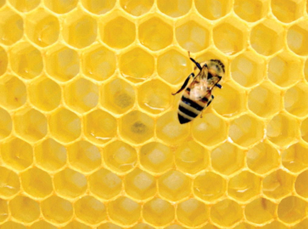
The solution to this problem is reasonably incontrovertible. Bees make honeycombs using eight parts of honey to one part of wax secreted from their own bodies. The honeycomb provides storage space for honey. It follows that they need maximum storage space for each unit of beeswax. Put another way they want to have maximum “bang for buck.” The storage space needs to be made up of identical interlinked units that are two-dimensionally symmetrical. It turns out that there are only three possible shapes that will satisfy this criterion: squares, equilateral triangles and regular hexagons. Fig. 2 presents these three shapes as interlinked arrays. This introduces the concept of models which are widely used in science because they simplify any calculations that have to be made.
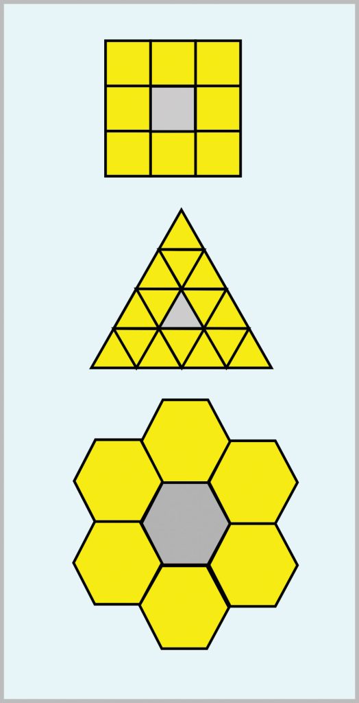
The “bang for buck” efficiency of the three alternative shapes can be deduced by simple calculations using the three greyed units. Let us assume that each straight side has the same length of 1 unit.
(1) Square
The area of a square of unit side is the square of its side length, therefore:
Area = 1.00
All four sides of the square contribute to a neighbouring square. The square’s area of 1.00 has therefore consumed only two sides. Hence we have that:
Square storage efficiency = 0.500
(2) Equilateral Triangle
The area of an equilateral triangle of unit side length is given by:
Area = 30.5/4 = 0.433
All three sides of the equilateral triangle contribute to a neighbouring triangle. The area of 0.433 has therefore consumed 1½ straight sides so that equilateral triangular storage efficiency is given by:
Equilateral triangle storage efficiency = 0.433/1.5 = 0.289
We see that the triangular storage efficiency is much lower than that of square storage efficiency.
(3) Regular Hexagon
The area of a regular hexagon of unit side length is given by:
Area = 31.5/2 = 2.598
All six sides of the regular hexagon contribute to a neighbouring hexagon.
The area 2.598 has consumed three straight sides so that regular hexagon storage efficiency is given by:
Regular hexagon storage efficiency = 2.598/3 = 0.866
We see that regular hexagon storage efficiency is much higher than that of square storage efficiency and very much higher than that of equilateral triangle storage efficiency.
Bees worked this out 100 million years ago!
Metal Packing Efficiency
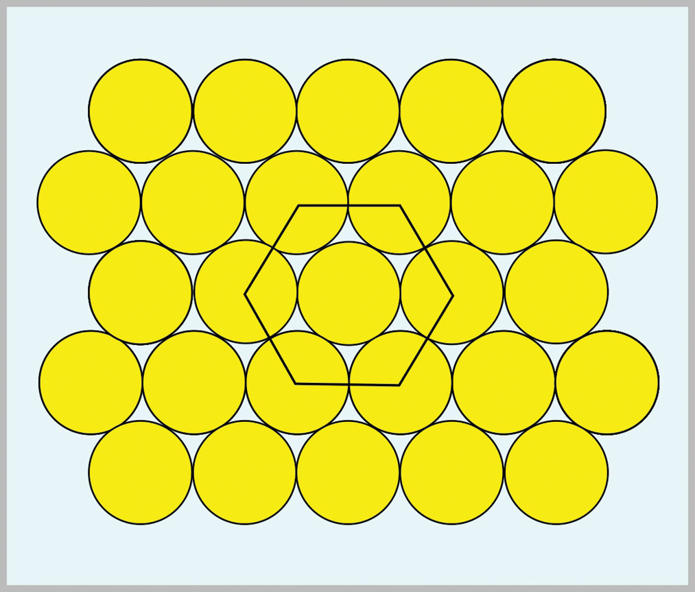
The three common metal crystal structures are body-centered-cubic (b.c.c.), face-centered-cubic (f.c.c.) and close-packed hexagonal (c.p.h.). F.c.c. and c.p.h metals both contain close-packed planes of ions. These close-packed planes correspond to maximum packing efficiency. Their packing is illustrated by fig. 3 in which a hexagon has been inscribed. It took until the 20th Century before Sir Lawrence Bragg, using x-ray diffraction, was able to discover close-packed planes.
Why are Snowflakes Sometimes Large and Sometimes Small?
A solution to this problem can be found by employing nucleation and growth theory. This theory has numerous applications such as explaining the properties of heat-treated metals.
Whenever a phase change takes place, such as freezing of water or pearlite formation in steels, nucleation and growth are the controlling factors. These can be regarded as competitors. New particles are trying to be nucleated while growth is competing to use the available phase change energy. Temperature has opposite effects on nucleation and growth rates which is the key to explaining the phenomenon. Fig. 4 is a schematic representation of the effect of temperature on competing nucleation and growth rates. The axes are deliberately non-dimensional because the effects apply universally.
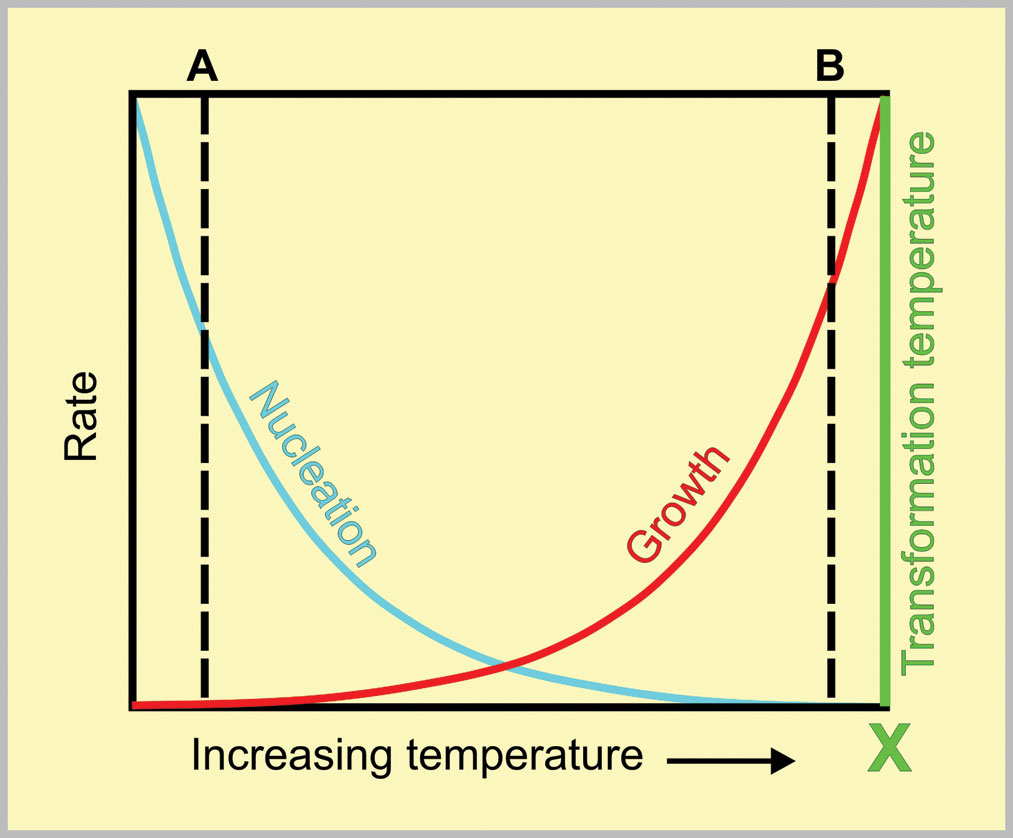
Consider the current problem of water freezing to form snowflakes. The temperature marked X in fig. 4 would then be 0˚C. If the air temperature was well below 0˚C (A in fig. 4), the nucleation rate would be very high but the growth rate would be very low — hence we get small snowflakes, Conversely, if the air temperature was only just below 0˚C (B in fig. 4), the nucleation rate would be very low but the growth rate would be very high, leading to large snowflakes.
Large snowflakes are only just below their melting point. Squeezing a handful injects sufficient energy for some melting to take place at myriad contact points. Immediate re-freezing at these points gives rise to a usable snowball. Small snowflakes, well below their melting point, do not respond by melting and re-freezing on squeezing, leaving one with a handful of powder.
Why Will a Glass of Warm Water Solidify More Quickly Than an Identical Glass of Cold Water When Placed Together in a Freezer?
This is a popular puzzle question first posed by Mpemba in 1963 whilst in Form 3 of Magamba Secondary School, Tanganyika. The headmaster had invited Dr. Denis Osborne from the University College in Dar es Salaam to give a lecture on physics. After the lecture, Mpemba asked the question, “If you take two similar containers with equal volumes of water, one at 35˚C (95˚F) and the other at 100˚C (212˚F), and put them into a freezer, why does the one that started at 100˚C (212˚F) freeze first?” He was ridiculed by his classmates and teacher. Osborne, however, later experimented on the proposition back at his workplace and confirmed Mpemba’s finding.
The fact that warm water can freeze faster than cold water has been known for thousands of years, being first recorded by Aristotle and later studied by many scientists including Bacon and Descartes. No generally accepted explanation for this anomalous behaviour has, however, been put forward so here goes with my own!
The heat that has to be extracted from the water is in two parts. Firstly that for lowering the water’s temperature to its freezing point and secondly that required to extract the latent heat of freezing. If the warm water was 50˚C above the temperature of the cold water then 50 more calories per cc would be required to be extracted by the freezer than would be required for the cold water before freezing could take place. This amount is, however, dwarfed by the magnitude of the latent heat for freezing the water. Rounding up this magnitude we get 350 calories per cc — freezing therefore requires about seven times the heat extraction needed for simply cooling the water.
Figs. 5 and 6, drawn to the same scale, represent the different stages anticipated for glasses of cold and warm water when placed together in a freezer.
The liquid cooling stage, 0 – A, for the warm water must be longer than that for the cold water. This time difference is much less than simply the initial temperature difference because of the stronger convection currents in warm water. The freezing stage will, however, be much shorter for the warm water than for the cold water!
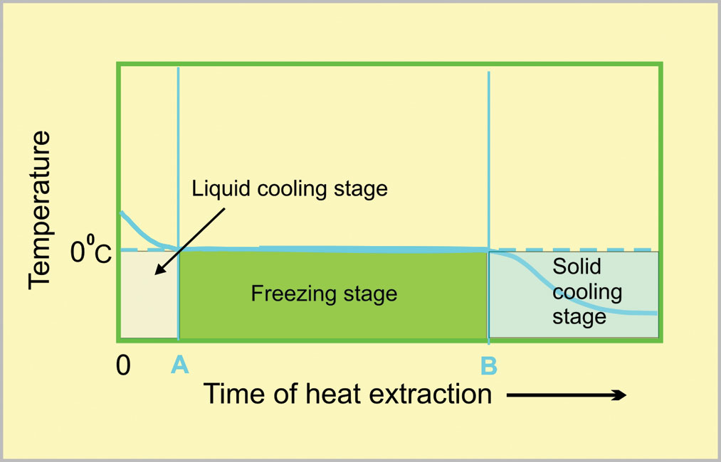
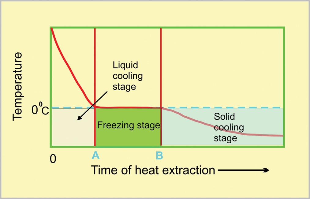
During the freezing stage, ice crystals are being nucleated and subsequently grow. Ice crystals can only nucleate slowly on the outside of a warm water glass — the warmth preventing the temperature from falling much below the freezing point. These crystals can, however, grow inwards quickly because the water temperature is being kept just below its freezing point. This results in a short freezing stage. For the cold water, ice crystals form rapidly on the outside of the glass because its temperature is being reduced well below the freezing point. These myriads of tiny crystals can, however, only grow slowly. This results in a much shorter freezing stage. Hence, the overall time for solidification, O – B, is shorter for the glass of warm water than it is for the glass of cold water.
NUCLEUS FORMATION AND GROWTH
Nucleation and growth controls the properties of all of the metals used by shot peeners. They go together like the proverbial “horse and carriage.”
Nucleus Formation
Metal atoms are very reluctant to collectively change from one state to another. There has to be a sufficient driving force available if a different state particle is to nucleate. Hot steel exists as a face-centered-cubic arrangement of ions. The steel has to be cooled sufficiently for the ions to form nuclei that have a body-centred-cubic arrangement. Solid-to-solid changes of state are the essence of metal heat treatment.
The surface of a nucleus corresponds to a negative energy force whereas the inside corresponds to a positive energy force. If the positive energy is greater than the negative energy, the nucleus will be stable. If smaller, then it will be unstable. The ratio of energies depends on the particle radius as depicted in fig. 7. Particle A will be unstable (negative energy being greater than the positive energy) whereas particle B will be stable (positive energy exceeding negative energy).
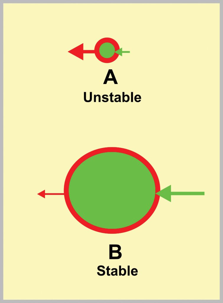
It is worth noting that spheres have the smallest surface area-to-core volume ratio of any physical shape. When cast steel shot is manufactured, a powerful water jet blasts into a stream of liquid steel. Myriads of solid particles are formed that minimize the ratio by forming spheres. The Earth and planets approach sphericity.
Nucleus Growth
Once a nucleus has reached a stable size it has a natural tendency to grow. The precise mechanism involved depends upon the state change — gaseous-to-solid, liquid-to-solid or solid-to-solid. Gaseous-to-solid, liquid-to-solid and solid-to-solid particle growth all follow the same basic principle — reducing energy by increasing the interior/surface energy ratio.
The most important example of nucleus growth is that involved in the formation of the planets. Gaseous matter is attracted to their surfaces by gravity. Once deposited on a surface, matter reduces its energy. Heat treatment examples include precipitate particle growth and austenite coarsening. Both are speeded up by raising the temperature.
GRAPHICAL REPRESENTATION
Scientific principles are involved in all of the graphs used by shot peeners — for example, in peening intensity curves, residual stress profiles and shot size distributions.
Peening Intensity
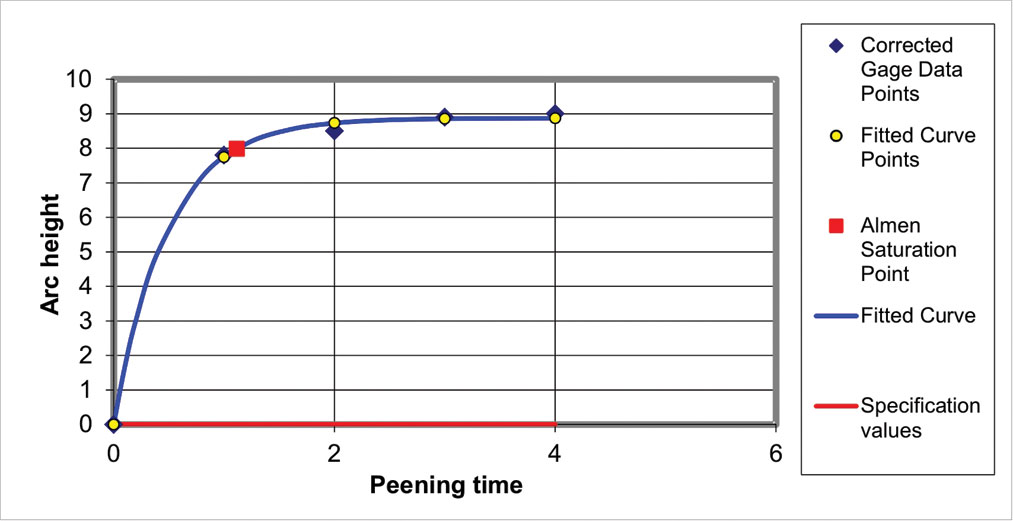
Curve-fitting is an essential feature of computer-based peening intensity estimation. We first decide on an appropriate equation for the curve and then employ a program to fit the curve normally using a technique called “Least Squares”. Fig. 8 is a typical Solver Suite peening intensity curve that uses a two-parameter exponential equation. A key feature of the Solver Suite of programs is the RMS value. This tells us, quantitatively, by how much data values deviate from the fitted curve. For the example given as fig. 8 the RMS value for the residuals (RMS-R) is 0.14 which is excellent.
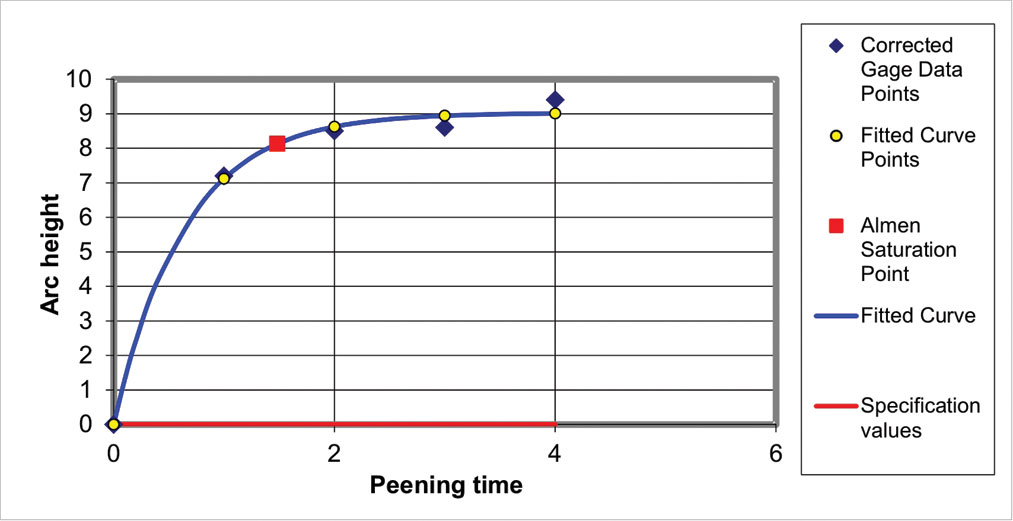
If a repeat set of data produced using the same conditions gave a much higher RMS value, we should investigate the reason such as faulty equipment, operator error, peening intensity fluctuation, etc. A typical repeat set is shown in fig. 9.
Residual Stress Profiles
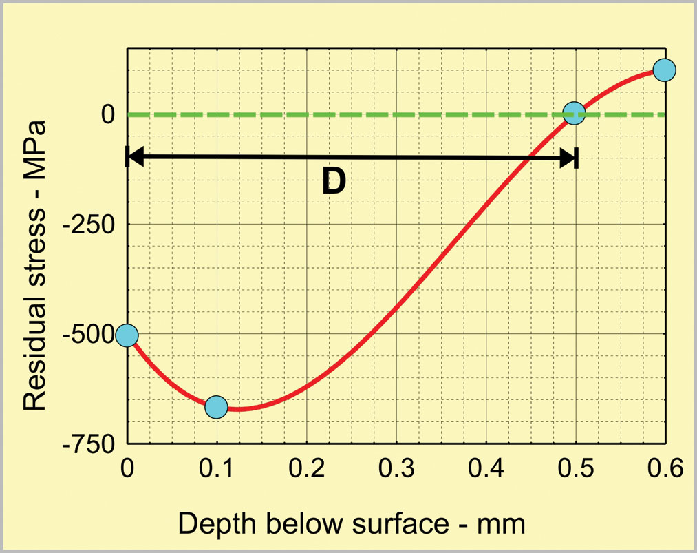
Residual stress profiles are another form of graphical representation that is familiar to shot peeners. Their shape is quite different from that of a peening intensity curve. Fig. 10 is taken from an early article in this series (“Curve Fitting for Shot Peening Data Analysis”, Spring, 2002). The scientific application here takes the form of modelling. Instead of using actual data, a simple cubic equation is employed. This particular model represents the known shape of residual stress profiles but is based on four assumptions:
- The level of surface compressive stress is half the yield strength, Y, of the as-peened material.
- The maximum level of compressive stress is two-thirds of Y and occurs at 20% of the depth of compressed material, D.
- A balancing tensile stress of 10% of Y is reached at 1.2D.
- A cubic polynomial interpolation will be appropriate.
Models are a useful scientific application because they simplify comparisons between actual and expected data distributions. A useful guide when perusing graphical representations is to employ EVA (Expected Versus Actual). Compare one’s expectation for a fitted curve versus the actual curve.
Shot Size Distributions
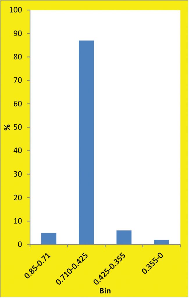
Specifications, such as SAE J444 and AMS 2431, nominate cast steel shot sizes in terms of sieving results. If we are simply trying to comply with specifications, histograms would not normally be constructed. Histograms can, however, be used to demonstrate shot size distribution. Because of the nature of sieve data, ordinary graphs are inappropriate.
The universal availability of Excel simplifies the task of producing histograms. As an example, consider the Excel histogram shown as fig. 11. A sample of S170 cast steel shot was tested for conformity with J444. Percentage weights on 0.850, 0.710, 0.425 and 0.355 mm sieves were 0, 5, 87, and 6% respectively which satisfies J444 requirements. Each column in the histogram represents the contents of a “bin”. Each bin contains a range of shot sizes — for example, everything between 0.85 and 0.71 mm for the first bin. The individual sieve results are therefore entered as separate bin values.
The example shown as fig. 11 does not, however, tell us very much about the size distribution within the sample. For scientific study we would need to produce a set of bin values involving a larger number of sieve sizes such as 0.85, 0.75, 0.65, 0.55, 0.45 and 0.35 mm. An alternative approach would be to use image analysis.
DISCUSSION
This article has attempted to show how science can be applied to explain a variety of problems. Classically, explanations of major problems evolve in stages, starting with a hypothesis, using data to then provide a theory and finally generating a law that is universally acceptable — as with the Law of Gravity. The appliance of science to explain observed experimental features does not, however, always meet with universal accord as Galileo found out to his cost.